Δ to Y Network Conversion

Δ to Y (π to T) Network Conversion

Many circuits contain sub-circuits comprising of a three terminal network connected in one of two ways:

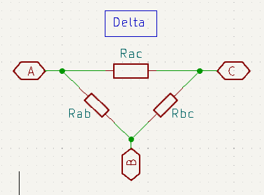
• The Delta (Δ) network – sometimes called a Pi (π) network depending upon how it is draw in the schematic.
• The ‘Y’ network – sometimes called a ‘T’ network depending upon how it is drawn in the schematic.

The Δ (or π) and Y (or T) networks can be configured to be electrically identical to each other. However, depending upon context one may be simpler to analyse than the other. Therefor it can be handy to know how to convert one type of network in to the other.

This article details how to derive the equations necessary to convert from a Delta (∆) [sometimes called a Pi (π)] network to a ‘Y’ [sometimes called a ‘T’] network. You could just memorise the final set of equations, though they look quite complex at first sight. For this reason I find it better to understand how the transforming equations are derived.

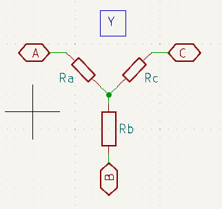
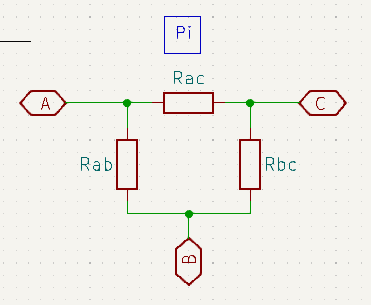
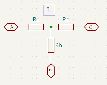
First of all let me emphasise that the Delta and Pi configurations are identical in every way, except for a minor difference in how they are drawn. Similarly, the ‘Y’ and ‘T’ are identical to each other in all but a minor presentation style.

In practice you will most often see the Pi and ‘T’ styles in schematic drawings. The reason for this is mostly down to the fact that a lot of CAD schematic capture packages make it difficult to rotate components at anything other multiples of 90 degrees. It can usually be done (as you can see above), however it is usually much quicker to lay out the Pi and ‘T’ configurations in the schematic editor.

Δ to ‘Y’ Conversion

We can derive a set of equations for the resistance seen looking in to the network between any two combinations of the terminals: AB, AC, and BC. We can do this for both the Delta and the ‘Y’ networks. So let’s start by doing that:

Since the Δ and ‘Y’ networks look electrically identical from the outside, we can expand out the series // parallel shorthand used above and say that each equation on the left column is equal to the corresponding equation in the right column:

\(AB = \frac{R_{ab}(R_{ac} + R_{bc})}{R_{ab} + R_{ac} + R_{bc}} = R_a + R_b\\\) \(AC = \frac{R_{ac}(R_{ab} + R_{bc})}{R_{ab} + R_{ac} + R_{bc}} = R_a + R_c\\\) \(BC = \frac{R_{bc}(R_{ab} + R_{ac})}{R_{ab} + R_{ac} + R_{bc}} = R_b + R_c\)

What we now have is a set of simultaneous equations¹ that we can solve to find R_a, R_b, and R_c in terms of R_ab, R_ac, and R_bc.

This is not intended to be a maths tutorial, so I am just going to run through solving for R_a manually and leave it to you to solve for R_b and R_c in a similar fashion. Alternatively, there are no shortage of online maths equation calculators these days (for example the excellent wolframalpha.com).

We’ll start by subtracting the third equation from the first to eliminate R_b

\((R_a + R_b) – (R_b + R_c) = \frac{R_{ab}(R_{ac} + R_{bc}) – R_{bc}(R_{ab} + R_{ac})}{R_{ab} + R_{ac} + R_{bc}} = R_b – R_c\\\)

Next we’ll add the second equation from this result to eliminate R_c. Leaving just R_a.

\((R_a – R_c) + (R_a + R_c) = \frac{R_{ab}(R_{ac} + R_{bc}) – R_{bc}(R_{ab} + R_{ac}) + R_{ac}(R_{ab} + R_{bc})}{R_{ab} + R_{ac} + R_{bc}} = 2R_a\\\)

Now expanding out the numerator on the right hand side we get:

\(2R_a = \frac{R_{ab}R_{ac} + R_{ab}R_{bc} – R_{ab}R_{bc} – R_{ac}R_{bc} + R_{ab}R_{ac} + R_{ac}R_{bc}}{R_{ab} + R_{ac} + R_{bc}}\\\)

Now simplifying we are left with:

\(2R_a = \frac{2R_{ab}R_{ac}}{R_{ab} + R_{ac} + R_{bc}}\\\)

and dividing both sides by 2 we get:

\(\frac{2R_a}{2} = \frac{2R_{ab}R_{ac}}{2(R_{ab} + R_{ac} + R_{bc})}\\\)

Which simplifies to:

\(R_a = \frac{R_{ab}R_{ac}}{R_{ab} + R_{ac} + R_{bc}}\)

The remaining equations for R_b and R_c are derived in a similar fashion. However, as I said before this not a maths tutorial so I will just list the final results below and leave you to do the derivation yourself (should you so wish).

\(R_a = \frac{R_{ab}R_{ac}}{R_{ab} + R_{ac} + R_{bc}}\\\) \(R_b = \frac{R_{ab}R_{bc}}{R_{ab} + R_{ac} + R_{bc}}\\\) \(R_c = \frac{R_{ac}R_{bc}}{R_{ab} + R_{ac} + R_{bc}}\)

Aide-Mémoire

Clearly no-one in their right mind wants to go through all of that each time the conversion is required, and memorising yet another three (non-trivial) equations is not an appealing prospect. However, things are not a bad as they first appear.

A closer inspection of the three equations while looking at the schematic diagrams reveals some key insights which may help:

• The equations look like a variation on the product over sum formula for two parallel resistors.
• The denominator for all three equations is the same: the sum of all the resistors in the delta network.
• Comparing the schematics we see that each resistor in the ‘Y’ network, could be seen as replacing a a pair of parallel resistors for the same location in the delta network.
• The numerator is the product of the two resistors that it replaces.

For convenience, the two network configurations are repeated below along with the three transformation equations to convert from the Delta on the left, to the ‘Y’ on the right.

\(R_a = \frac{R_{ab}R_{ac}}{R_{ab} + R_{ac} + R_{bc}}\\\) \(R_b = \frac{R_{ab}R_{bc}}{R_{ab} + R_{ac} + R_{bc}}\\\) \(R_c = \frac{R_{ac}R_{bc}}{R_{ab} + R_{ac} + R_{bc}}\)

---

Footnotes

1. If you need a reminder on how to solve systems of simultaneous linear equations. See here. ↩︎