Mesh Current Analysis

Mesh Current Analysis (a.k.a. Loop Analysis)

The motivation for Mesh Analysis is that sometimes you have a circuit which is too complicated to solve using a simplification method, such as superposition. Mesh analysis on the other hand will work for any circuit that has just resistors and voltage and or current sources in any configuration. The price you pay for that power and flexibility is that it can be quite an involved process, and will require the solving of multi-variable simultaneous equations at the end. However, that’s what calculators are for (you can also use one of the excellent online equation calculators such as Woolfram Alpha).

Having said that the technique is involved, it’s also relatively straight forward to understand. You start by identifying loops in the circuit and then use Kirchhoff’s Voltage Law along with Ohms Law to create equations describing each loop. Then solve those equations for the current and voltages in those loops.

Example Analysis

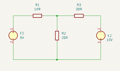
To keep this example as clear and straight forward as possible I’m going to use a very simple circuit, which could easily be solved by one of the simpler techniques such as superposition. However, the process and steps are the same, there would just be more loops to analyse.

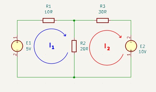
Step 1 – Identify and label the loops

Identify and label the loops (hence this technique is sometimes known as Loop Analysis) and arbitrarily assign a direction for the current in each loop (and we use conventional current flow, not electron flow). It is normal to choose a clockwise direction for all the loops, as at this point we don’t actually know for certain which way it is flowing. For the calculations it doesn’t matter, if we were wrong then it will just result in a negative answer which let’s us know that current actually flows the other way round the loop.

An important point to note here is that each loop is an inner loop. You can’t have a mesh inside another mesh. However, together all the inner loops cover every component through which current flows. Though you can, and will, have meshes in adjacent loops that pass through a common component at the boundary between the loops. In fact this is where the name mesh analysis comes from as the loops mesh together.

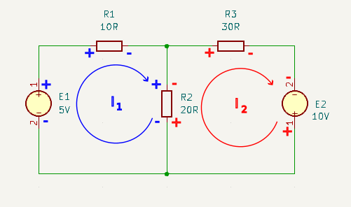
Step 2 – Mark polarities for every component

For each loop that was identified mark the ‘+’ and ‘-‘ polarity of each component. This is the polarity implied by the chosen current direction for anything that is a voltage drop (so ‘+’ on the input, and ‘-‘ on the output side). Voltage and current sources on the other hand retain their actual polarities (‘-‘ on the input, and ‘+’ on the output side).

Note this means that components which are on the boundary between two loops may have two differing sets of polarities (one associated with each loop). This is fine as the current through that component is the sum of the currents contributed from each loop.

Step 3 – Create a KVL equation for each loop

For each loop that has been identified, choose a starting point and generate a KVL equation in terms of the voltage sources and voltage drops within each loop. Don’t worry that you don’t know the actual voltage drops, just write them in terms of Ohms Law equations (V = I.R where ‘I’ will be written as ‘I_n‘, and ‘n’ will be the loop number).

The only gotcha here is that the current for those resistors that are in two loops, need to have both currents included in the equation and the polarity for each loop current has to be accounted for. In our example circuit R₂ is shared by both I₁ and I₂. The voltage drop is therefor R₂ * (I₁ – I₂) because the currents are opposing each other.

Don’t worry the magic of simultaneous equations will resolve those variables later.

For our example I am choosing to start at the bottom left corner for I₁ and in the bottom right corner for I₂ then:

KVL for I₁

\(E_1 – I_1.R_1 – R_2.(I_1 – I_2) = 0 \\\) \(5 – 10.I_1 – 20.(I_1 – I_2) = 0 \\\) \(5 – 10.I_1 – 20.I_1 + 20.I_2 = 0 \\\) \(-30.I_1 + 20.I_2 = -5 \\\) \(30.I_1 – 20.I_2 = 5 \\\)

KVL for I₂

\(-R_2.(I_2 – I_1) – R_3.I_2 + E2 = 0 \\\) \(-20.(I_2 – I_1) – 30.I_2 + 10 = 0 \\\) \(-20.I_2 + 20.I_1 – 30.I_2 + 10 = 0 \\\) \(20.I_1 – 50.I_2 = -10 \\\) \(-20.I_1 + 50.I_2 = 10 \)

Step 4 – Solve the equations derived in step 3

This is just a simple simultaneous equation to solve for two unknown variables. I’m not going to show how to do that because there is no point these days. Just use either your calculator or an online equation solver such as Wolfram Alpha.

Just type the equations in to your chosen equation solving tool and out will pop the answer. Which in our case is:

We can’t use I₁ and I₂ as variable names because it might think they are complex numbers, so we will substitute ‘a’ for ‘I₁‘ and ‘b’ for ‘I₂‘.

So typing 30a – 20b = 5, -20a + 50b = 10 in to www.wolframalpha.com returns:

\(a = \frac{9}{22}, b = \frac{4}{11} \\\)

Wolfram Alpha tries to give a precise answer which is why it is given as a fraction. However, for our purposes we can use an ordinary calculator to convert that into decimals giving:

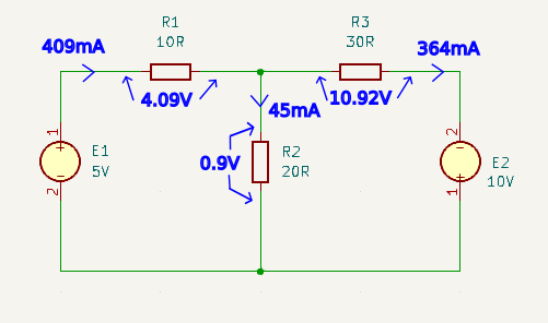
\(I_1 = \frac{9}{22} = 0.40909A \approx 409mA \\\) \(I_2 = \frac{4}{11} = 0.363636A \approx 364mA\)

Step 5 – Find all Voltage across & current through all components

Now that we know the value of the current for each loop, we can calculate the voltage across, and current through, all the components.

Let’ start by doing the calculations for the I1 loop:

\(V_{R1} = I_1.R_1 = 0.409 * 10 = 4.09V \\\)

Let’s start by assuming that the direction of current through R₂ is the same as we defined for I₁. Then:

\(I_{R2} = I_1 – I_2 = 0.409 – 0.364 = 0.045A = 45mA \\\)

Which is a positive value indicating that we guessed correctly about the direction of current through that resistor. The current (45mA) is flowing from top to bottom. So given our chosen direction of current the voltage across R2 will be a drop:

\(V_{R2} = I_{R2}.R_2 = 0.045 * 20 = 0.9V \\\)

So cross checking loop I1 with KVL we get:

\(E_1 – V_{R1} – V_{R2} = 0V \\\) \(5V – 4.09V – 0.9V = 0.01V \\\)

Which allowing for the rounding that we did in approximating currents is correct.

Now let’s do the same for the I2 loop:

\(V_{R3} = I_2.R_3 = 0.364 * 30 = 10.92V \\\)

Remember that we already established that the direction of current through R2 is in opposition to I2, then as far as the I2 loop goes, V_{R2} is a generator of voltage so. Checking our answers using KVL gives us:

\(V_{R2} – V_{R3} + E_2 = 0V \\\) \(0.9V – 10.92V + 10V = -0.02V \\\)

Which after accounting for rounding errors is correct.

Summary

After taking in to account rounding errors during our calculations we can be sure that our analysis yields the following results:

\(E_1 = 5V \\\) \(I_{E1} = 409mA \\\)

\(I_{R1} = 409mA \) left to right

\(V_{R1} = 4.09V \\\)

\(I_{R2} = 45mA \) top to bottom

\(V_{R2} = 0.9V \)

\(I_{R3} = 364mA \) left to right

\(V_{R3} = 10.92V \\\) \(E_2 = 10V \\\) \(I_{E2} = 364mA \\\)