- What is electricity?
- Resistance, Conductance & Ohms Law
- Practical Resistors
- Power and Joules Law
- Maximum Power Transfer Theorem
- Series Resistors and Voltage Dividers
- Kirchhoff’s Voltage Law (KVL)
- Parallel Resistors and Current Dividers
- Kirchhoff’s Current Law (KCL)
- Δ to Y Network Conversion
- Y to Δ Network Conversion
- Voltage and Current Sources
- Thevenin’s Theorem
- Norton’s Theorem
- Millman’s Theorem
- Superposition Theorem
- Mesh Current Analysis
- Nodal Analysis
- Capacitance
- Series & Parallel Capacitors
- Practical Capacitors
- Inductors
- Series & Parallel Inductors
- Practical Inductors
Power and Joules Law
Intuitively we all know what power is. A more powerful motor can turn a heavier load, or turn it faster; A more powerful torch will shine brighter; A more powerful heater will heat a larger volume faster. What these scenarios all have in common is to show that more power equates to more work being done in a given time. Since work is measured in joules, and time in seconds we get:
\(Power = \frac{work}{time} = \frac{joules}{second}\)
and Joules first law tells us that:
The power of heating generated by an electrical conductor equals the product of it’s resistance and the square of it’s current.
Or, in modern terms:
\(Power = I^2.R\)
So how do these things mesh together (we are talking DC steady state here). Well, power is measured in watts (symbol W) and having the designation P. Now consider that volts are in fact joules per coulomb, and that current is in fact coulombs per second. Also, from Ohms law we know that voltage is the product of current and resistance. So here is how the equation for power can be derived from a combination of Ohms and Joules laws:
\(P = I^2.R = I.I.R\) then substituting V for I * R
\(P = V.I\) then substituting joules/coulomb for V, and coulombs/second for I
\(P = \frac{joules}{coulomb} . \frac{coulombs}{second}\) and finally cancelling out the coulombs component
\(P = \frac{joules}{second} = Power\) in watts
Since we also know from Ohms law that current is voltage over resistance, we can derive a third form of the power equation:
\(P = V.I\) then substituting V/R for I
\(P = V.\frac{V}{R}\) and multiplying out the V component to get
\(P = \frac{V^2}{R}\)
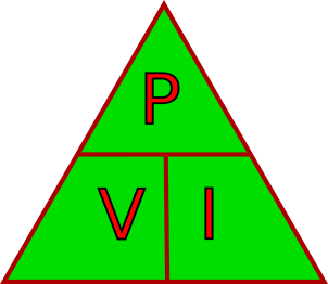
As an alternative, many people find that an aide-mémoire, similar to the Ohms law triangle helpful. Just place a thumb over the value of interest, and the remaining letters show how to obtain that value. For example, to find the power cover P and what remains is V x I. Alternatively to find the current, cover I and what remains is P over V, etc.
Summary
To summarise, when we put all this together we get a grande total of 12 equations for all the different variations of Ohms and Joules laws:
\(V = I.R\\\)
\(I = \frac{V}{R}\\\)
\(R = \frac{V}{I}\\\)
\(P = V.I\\\)
\(V = \frac{P}{I}\\\)
\(I = \frac{P}{V}\\\)
\(P = I^2.R\\\)
\(R = \frac{P}{I^2}\\\)
\(I = \sqrt{\frac{P}{R}}\\\)
\(P = \frac{V^2}{R}\\\)
\(R = \frac{V^2}{P}\\\)
\(V = \sqrt{P.R}\\\)
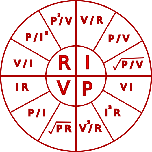
Some people also use a wheel similar to the one below as an aide-mémoire. Though to be honest I don’t recommend it. It seems to me far easier to remember just two simple equations (V = IR and P = VI) then just derive any of the other versions by transposition and substitution as you need them. However, just in case it is of help to you, here is a version of said wheel:
System Efficiency
Often when analysing a system it is important to know how efficient it is. In electrical systems this is usually a measure of proportion of the proportion of the total power used by the circuit appears in it’s output. It is normally expressed as a percentage:
\(Efficiency = \frac{Power_{out}}{Power_{in}} * 100\)